Welcome to Ocelli!

Ocelli (singular Ocellus, Latin: little eye) – simple eyes found in many insects in triplets. Their function is to navigate insects during the day or to detect movement.

Ocelli is an open-source Python library with computational tools for preprocessing, analyzing, and plotting developmental multimodal single-cell data. Ocelli’s functionality includes the following:

• modeling developmental multimodal processes with Multimodal Diffusion Maps,

• reducing data dimensionality with ForceAtlas2 and UMAP,

• calculating z-scores of gene signatures,

• producting 2D and interactive 3D plots.

Ocelli can be easily added to known single cell analysis pipelines through integration with AnnData data structure.

This series of tutorials introduces a spectrum of Ocelli’s functionality and applications. Ocelli is designed for analyzing multimodal data when each cell has entries from each modality. In tutorial 1, you will build your intuition by exploring simulated data. You will then proceed to multimodal single-cell data from hair follicle (tutorials 2 and 3), BMMCs (tutorials 4, 5, and 6), including modalities such as gene expression (RNA-seq), chromatin accessibility (ATAC-seq), protein epitopes, and histone modifications (H3K27ac and H3K27me3). In tutorial 7, you will employ Ocelli to explore unimodal pancreatic endocrinogenesis and cell reprogramming datasets.

After these tutorials, you should be able to:

• explore single-cell developmental multimodal data,

• understand the benefits of joint analysis and visualization of multimodal data,

• construct Multimodal Diffusion Maps embeddings of simulated and experimental data and visualize them using Ocelli.

Tutorial 1: Simulated data

Simulated data I: A binary tree

A modality refers to an experimentally measured set of genome-wide features. For example, scRNA-seq is a single-cell modality in which counts of RNA molecules are measured in single cells, represented by a cell-by-gene count matrix encoding gene expression. The higher the value in the count matrix, the more expressed a gene is in a cell. However, a wide range of biological information is lost when analyzing only the transcriptome. A simplistic version of the central dogma of molecular biology states that DNA makes RNA, and RNA makes protein. As a result, when looking solely at RNA levels, you omit information hidden in DNA and proteins. To understand biological processes at a molecular level, you must interpret multimodal, not unimodal information.

This tutorial introduces multimodal analysis based on simulated data, available for download on figshare. Analysis of single-cell data is discussed in subsequent tutorials.

Download simulated data and import necessary packages. Ocelli has four modules: oci.read (data reading), oci.pp (data preprocessing), oci.tl (analysis tools), and oci.pl (plotting). The workflow typically consists of multiple calls on an anndata.AnnData object.

import os
os.environ['TF_CPP_MIN_LOG_LEVEL'] = '2'

import ocelli as oci
from matplotlib.colors import LinearSegmentedColormap

! wget --content-disposition https://figshare.com/ndownloader/articles/28131449/versions/1
! unzip -o 28131449.zip
! rm 28131449.zip

--2025-01-29 18:29:40--  https://figshare.com/ndownloader/articles/28131449/versions/1
54.170.28.5, 52.17.87.113, 2a05:d018:1f4:d003:6dec:dfbb:5bc1:fcf0, ...
Connecting to figshare.com (figshare.com)|54.170.28.5|:443... connected.
HTTP request sent, awaiting response... 200 OK
Length: 764590 (747K) [application/zip]
Saving to: ‘28131449.zip’

28131449.zip        100%[===================>] 746.67K  3.38MB/s    in 0.2s

2025-01-29 18:29:40 (3.38 MB/s) - ‘28131449.zip’ saved [764590/764590]

Archive:  28131449.zip
 extracting: simulated_data_I.h5ad
 extracting: simulated_data_II.h5ad

Exploring single modalities

Load the first simulated dataset. Ocelli uses AnnData, an annotated data structure. If you need to familiarize yourself with it, we recommend glancing at its documentation.

simul = oci.read.h5ad('simulated_data_I.h5ad')

simul

AnnData object with n_obs × n_vars = 6000 × 1
    obs: 'type', 'pseudotime'
    uns: 'modalities'
    obsm: 'modality0', 'modality1', 'modality2'

The loaded dataset has three modalities (modality0, modality1, and modality2) stored in simul.obsm and represented as arrays in which rows and columns correspond to observations and features, respectively. Note that i-th row in all modalities corresponds to the same observation. Each modality has 6,000 3-dimensional observations.

for modality in ['modality0', 'modality1', 'modality2']:
    print('Shape of {} array: {}'.format(modality,
                                         simul.obsm[modality].shape))

Shape of modality0 array: (6000, 3)
Shape of modality1 array: (6000, 3)
Shape of modality2 array: (6000, 3)

simul.uns['modalities'] specifies simul.obsm keys that store modality arrays.

simul.uns['modalities']

array(['modality0', 'modality1', 'modality2'], dtype=object)

simul.obs is a pandas.DataFrame with observation metadata.

simul.obs

	type	pseudotime
0	A	0.000000
1	A	0.000333
2	A	0.000667
3	A	0.001000
4	A	0.001334
...	...	...
5995	F	0.998666
5996	F	0.999000
5997	F	0.999333
5998	F	0.999667
5999	F	1.000000

6000 rows × 2 columns

Observations are grouped into six types A-F (simul.obs['type']) and ordered along a developmental pseudotime (simul.obs['pseudotime']). simul.var, analogically, stores feature metadata.

Ocelli can produce scatter plots with Matplotlib or interactive plots with Plotly. The presented tutorials will show only static plots due to the compatibility issues between interactive plots and online documentation.

You can visualize each of the 3D modalities in two ways:

1. as a 3D interactive plot,

#oci.pl.scatter_interactive(simul, x='modality0', c='type', s=2, cdiscrete=cdict, showaxes=True)

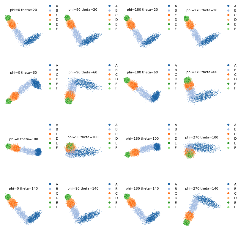
2. or as a 2D projection. For projecting 3D data onto 2D planes, you can use Ocelli’s oci.tl.projection function. It projects 3D data onto planes defined by their normal vectors (vectors perpendicular to the plane) oriented using polar coordinates phi (range: 0-360 degrees) and theta (range: 0-180 degrees). For quick look at multiple projection planes, use oci.pl.projections.

# define plotting colors for observation types
cdict = {'A': '#1a62a5',
         'B': '#a0bae2',
         'C': '#fd6910',
         'D': '#fdac65',
         'E': '#289322',
         'F': '#89db77'}

oci.pl.projections(simul, x='modality0', c='type', phis=[0, 90, 180, 270],
                   thetas=[20, 60, 100, 140], cdict=cdict, s=1, fontsize=8,
                   figsize=(8, 8), showlegend=True, random_state=17)

Select a specific projection plane: phi=90 and theta=20.

oci.tl.projection(simul, x='modality0', phi=90, theta=20, random_state=17)
# oci.tl.projection saves the projection by default to simul.obsm['X_proj']

oci.pl.scatter(simul, x='X_proj', c='type', cdict=cdict, s=3, markerscale=2,
               fontsize=15, figsize=(7, 6), title='')

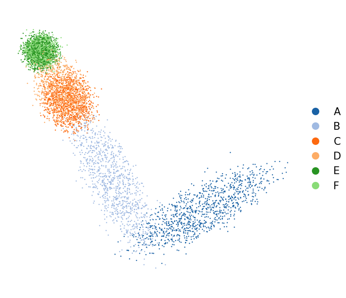
Observations form half of a binary tree with three branching points - each visible in a separate modality. modality0 splits apart types A and B, while types C, D, and E, F are mixed up. When looking only at modality0, it is impossible to understand the entirety of the underlying developmental process beyond A and B observations.

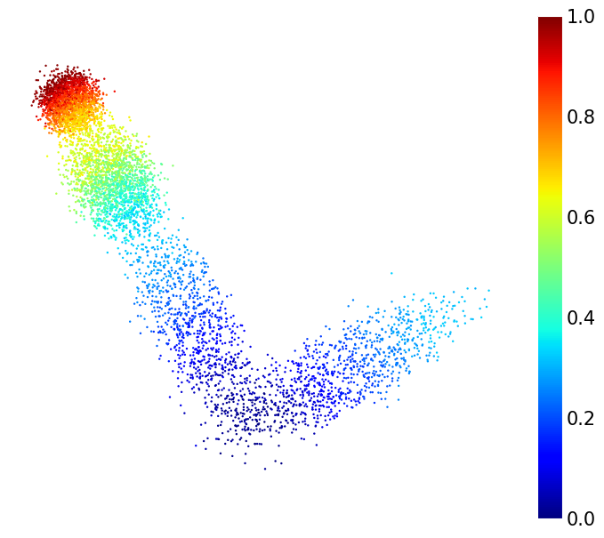
Observations are ordered along a pseudotime. The developmental process begins at the branching point of types A and B and proceeds further.

oci.pl.scatter(simul, x='X_proj', c='pseudotime', cmap='jet', s=3,
               markerscale=2, fontsize=15, figsize=(7, 6), title='')

Repeat the visualization steps for modality1.

oci.pl.projections(simul, x='modality1', c='type', phis=[0, 90, 180, 270],
                   thetas=[20, 60, 100, 140], cdict=cdict, s=1, fontsize=8,
                   figsize=(8, 8), showlegend=True, random_state=17)

Select a projection.

oci.tl.projection(simul, x='modality1', phi=0, theta=20, random_state=17)
oci.pl.scatter(simul, x='X_proj', c='type', s=3, markerscale=2, cdict=cdict,
               fontsize=15, figsize=(5, 6), title='')

oci.pl.scatter(simul, x='X_proj', c='pseudotime', cmap='jet', s=3,
               markerscale=2, fontsize=15, figsize=(5, 6), title='')

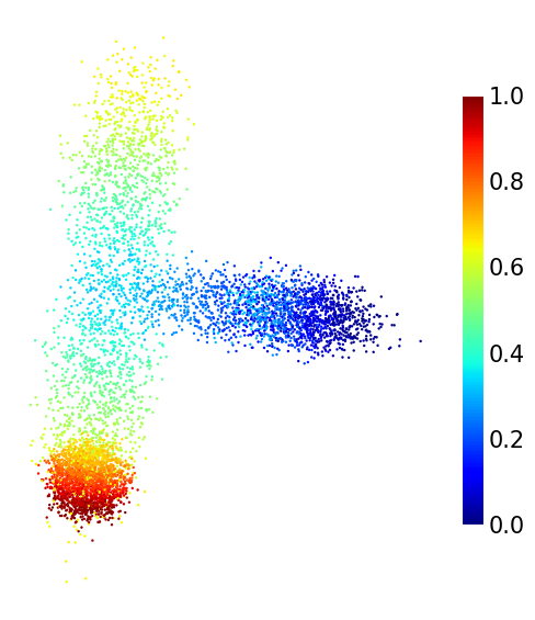
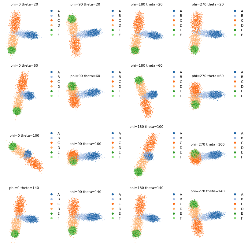
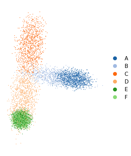
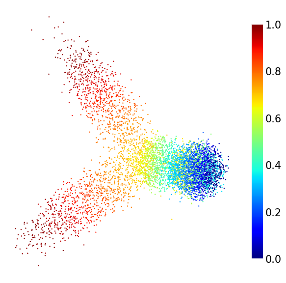
modality1 allows us to uncover lineages of types C and D, indistinguishable in modality0.

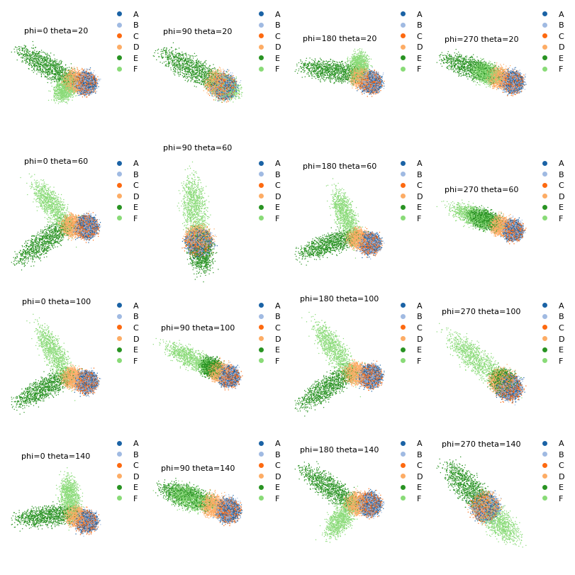
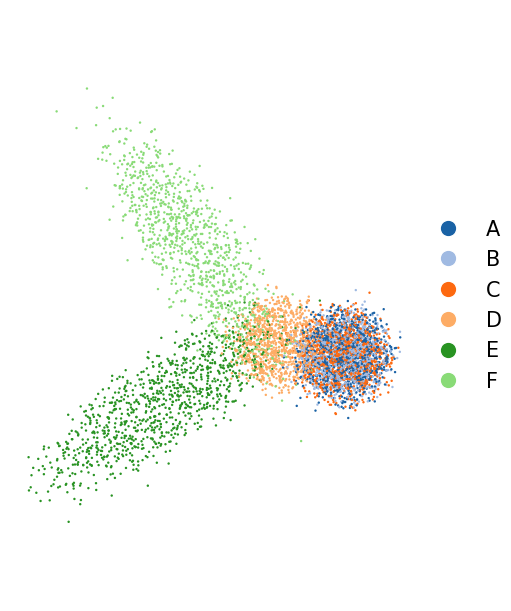
Similarly, modality2 reveals types E and F as separate lineages, unseen when looking at modality0 or modality1.

oci.pl.projections(simul, x='modality2', c='type', phis=[0, 90, 180, 270],
                   thetas=[20, 60, 100, 140], cdict=cdict, s=1, fontsize=8,
                   figsize=(8, 8), showlegend=True, random_state=17)

oci.tl.projection(simul, x='modality2', phi=180, theta=100, random_state=17)
oci.pl.scatter(simul, x='X_proj', c='type', s=3, markerscale=2, cdict=cdict,
               fontsize=15, figsize=(5, 6), title='')

oci.pl.scatter(simul, x='X_proj', c='pseudotime', s=3, markerscale=2,
               cmap='jet', fontsize=15, figsize=(6, 6), title='')

Multimodal Diffusion Maps

All above plots are unimodal - they do not visualize all levels of available information. Multimodal Diffusion Maps (MDM) is a diffusion-based algorithm for embedding multimodal data into a joint latent space. Using MDM with Ocelli can be split into three stages.

1. Finding observations’ nearest neighbors in the feature space across all modalities.

oci.pp.neighbors(simul, n_neighbors=20, n_jobs=50, verbose=True)

[modality0]     20 nearest neighbors calculated.
[modality1]     20 nearest neighbors calculated.
[modality2]     20 nearest neighbors calculated.

2. Calculating multimodal weights for each observation.

Multimodal weights form a distribution over modalities, each observation’s weights summing to 1. A higher weight indicates that the algorithm selected the modality as more informative about observation and its neighborhood than others.

Some Ocelli functions, including oci.tl.modality_weights, have probabilistic steps. You can set a value of a random_state parameter for the sake of reproducibility. If you omit this step, each run will result in marginally different outcomes, which is a natural effect in stochastic processes. Note that despite setting a random_state, result may be different on different processors.

oci.tl.modality_weights(simul, random_state=17, n_jobs=50, verbose=True)

2025-01-29 18:29:52,975 INFO worker.py:1518 -- Started a local Ray instance.

Multimodal weights estimated.

3. Calculating the MDM embedding.

The parameter n_components defines the dimensionality of the MDM latent embedding. A good practice is to explore different values for each dataset individually. MDM components are information-rich, but their quality decreases with increasing number of components.

Technical remark: below, ``unimodal_norm`` is ``False``. Use its default ``True`` value for single-cell data. ``unimodal_norm``’s value is changed here because the simulated 3D data is sampled from an artificial distribution, which is low-dimensional and dense. Single-cell data come from high-dimensional latent spaces of incomparable complexity that are properly normalized during data preprocessing (details in the following tutorials).

oci.tl.MDM(simul, n_components=10, unimodal_norm=False, random_state=17, n_jobs=50, verbose=True)

2025-01-29 18:29:58,646 INFO worker.py:1518 -- Started a local Ray instance.

[modality0]     Unimodal Markov chain calculated.
[modality1]     Unimodal Markov chain calculated.
[modality2]     Unimodal Markov chain calculated.
Multimodal Markov chain calculated.
Eigendecomposition finished.
10 Multimodal Diffusion Maps components calculated.

The resulting 10-dimensional MDM embedding represents a multimodal latent space from which the modeled developmental process originates. The embedding is saved to simul.obsm['X_mdm'].

Visualizing MDM components

Ocelli allows to visualize MDM embeddings with ForceAtlas2 or UMAP.

ForceAtlas2 is a force-directed layout algorithm for graph visualization. Running ForceAtlas2 with Ocelli requires three steps:

• finding nearest neighbors in the MDM latent space,

• computing the nearest neighbor graph,

• calculating the force-directed layout graph representation.

oci.pp.neighbors(simul, x=['X_mdm'], n_neighbors=30, n_jobs=50, verbose=True)
oci.tl.neighbors_graph(simul, x='X_mdm', n_edges=30, verbose=True)
oci.tl.fa2(simul, n_components=2, n_iter=5000, n_jobs=50, random_state=17)

[X_mdm] 30 nearest neighbors calculated.
Nearest neighbors-based graph constructed.

Jan 29, 2025 6:30:10 PM org.netbeans.modules.masterfs.watcher.Watcher getNotifierForPlatform
INFO: Native file watcher is disabled
Jan 29, 2025 6:30:11 PM org.gephi.io.processor.plugin.DefaultProcessor process
INFO: # Nodes loaded: 6,000 (6,000 added)
Jan 29, 2025 6:30:11 PM org.gephi.io.processor.plugin.DefaultProcessor process
INFO: # Edges loaded: 180,000 (108,678 added)

*************************25%
*************************50%
*************************75%
*************************100%
Time = 32.478s

Plot the resulting force-directed layout embedding (FLE).

oci.pl.scatter(simul, x='X_fa2', c='type', cdict=cdict, s=5, markerscale=2,
               fontsize=15, figsize=(6,6), title='')

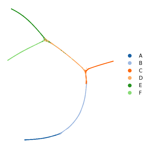
In the MDM latent space, all observation types A-F are separated with well-defined branching points. It is easy to trace all developmental lineages, which were impossible to spot together in unimodal exploration.

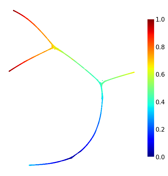
Moreover, the MDM representation preserves developmental pseudotime.

oci.pl.scatter(simul, x='X_fa2', c='pseudotime', cmap='jet', s=5, fontsize=15,
               figsize=(6,6), title='')

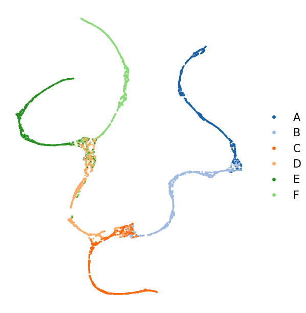
Alternatively, you can run UMAP. For well-connected data, we recommend ForceAtlas2, and for data with separate clusters, UMAP.

oci.tl.umap(simul, x='X_mdm', n_components=2, n_neighbors=20, min_dist=0.1,
            n_jobs=50, random_state=17)

oci.pl.scatter(simul, x='X_umap', c='type', cdict=cdict, s=5, fontsize=15,
               figsize=(6,6), title='')

Exploring modality weights

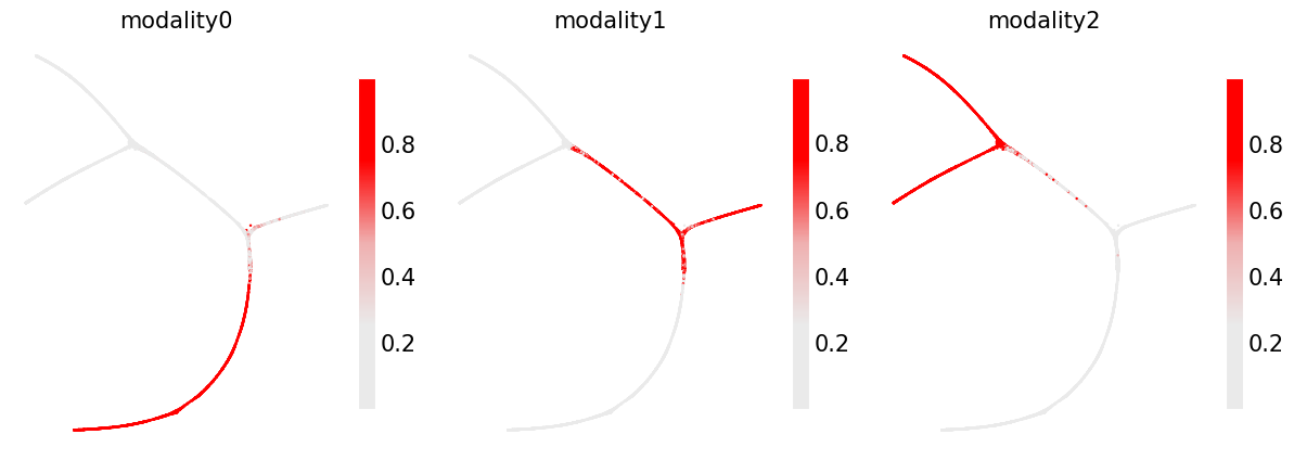
Calculated multimodal weights provide an explainable insight into the MDM’s training. They are saved to simul.obsm['weights'].

simul.obsm['weights']

	modality0	modality1	modality2
0	0.973592	0.025576	0.000832
1	0.989186	0.008797	0.002017
2	0.992478	0.006181	0.001341
3	0.967995	0.030422	0.001583
4	0.993608	0.004865	0.001527
...	...	...	...
5995	0.000107	0.000101	0.999793
5996	0.000115	0.000101	0.999784
5997	0.000117	0.000101	0.999782
5998	0.000159	0.000095	0.999746
5999	0.000148	0.000108	0.999744

6000 rows × 3 columns

You can examine the weight distribution concerning each observation type.

oci.pl.violin(simul, groups='type', values='weights', cdict=cdict, fontsize=15,
              figsize=(8, 6))

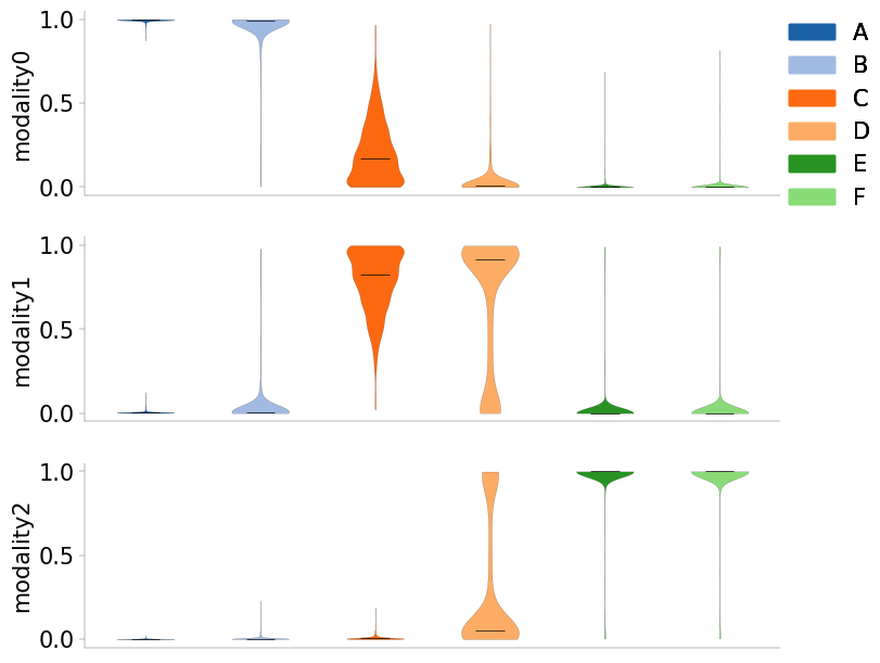
modality0 is dominant for types A and B, modality1 for types C and D, and modality2 for types E and F.

You can further visualize multimodal weights on scatter plots.

# define a custom colormap
cmap = LinearSegmentedColormap.from_list(
    'custom', ['#eaeaea', '#eaeaea', '#efb0b0', '#ff0000', '#ff0000'], N=256)

oci.pl.scatter(simul, x='X_fa2', c='weights', cmap=cmap,  s=3,
               fontsize=15, figsize=(12, 5))

The advantage of multiple modalities

Above, you investigated three modalities, each introducing a branching point starting two lineages. You created a joint multimodal representation capturing all developmental fates, inseparable by single modalities.

Now, you will further explore joint representations by limiting information fed to MDM. Run MDM on two modalities, e.g., modality0 and modality1. This way, you take away information about the separability of type E and F fates.

Change simul.uns['modalities'] so that MDM is trained on modality0 and modality1.

simul.uns['modalities'] = ['modality0', 'modality1']

Calculate multimodal weights and MDM components.

oci.tl.modality_weights(simul, random_state=17, n_jobs=50, verbose=True)
oci.tl.MDM(simul, n_components=10, unimodal_norm=False, random_state=17, n_jobs=50, verbose=True)

2025-01-29 18:31:15,602 INFO worker.py:1518 -- Started a local Ray instance.

Multimodal weights estimated.

2025-01-29 18:31:21,510 INFO worker.py:1518 -- Started a local Ray instance.

[modality0]     Unimodal Markov chain calculated.
[modality1]     Unimodal Markov chain calculated.
Multimodal Markov chain calculated.
Eigendecomposition finished.
10 Multimodal Diffusion Maps components calculated.

Create the nearest neighbor graph in the MDM latent space and compute FLE.

oci.pp.neighbors(simul, x=['X_mdm'], n_neighbors=30, n_jobs=50, verbose=True)
oci.tl.neighbors_graph(simul, x='X_mdm', n_edges=30, verbose=True)
oci.tl.fa2(simul, n_components=2, n_iter=5000, n_jobs=50, random_state=17)

[X_mdm] 30 nearest neighbors calculated.
Nearest neighbors-based graph constructed.

Jan 29, 2025 6:31:33 PM org.netbeans.modules.masterfs.watcher.Watcher getNotifierForPlatform
INFO: Native file watcher is disabled
Jan 29, 2025 6:31:33 PM org.gephi.io.processor.plugin.DefaultProcessor process
INFO: # Nodes loaded: 6,000 (6,000 added)
Jan 29, 2025 6:31:33 PM org.gephi.io.processor.plugin.DefaultProcessor process
INFO: # Edges loaded: 180,000 (107,431 added)

*************************25%
*************************50%
*************************75%
*************************100%
Time = 33.079s

oci.pl.scatter(simul, x='X_fa2', c='type', cdict=cdict, s=5, markerscale=2,
               fontsize=15, figsize=(6,6), title='')

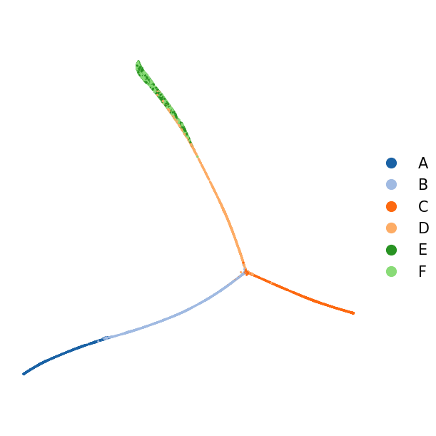
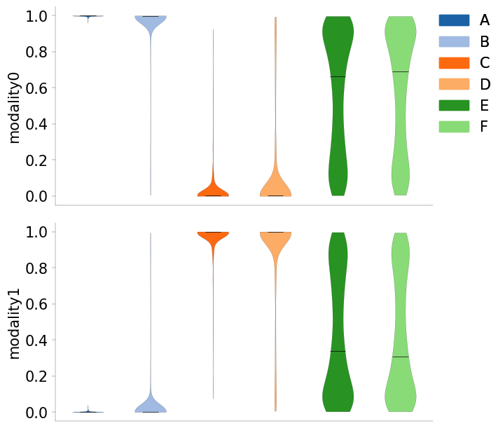
Developmental fates E and F from unused modality2 are mixed, while types well-separated in modality0 and modality1are correctly reconstructed. Multimodal weight distribution shows why this happens.

oci.pl.scatter(simul, x='X_fa2', c='weights', cmap=cmap, s=3,
               fontsize=15, figsize=(10, 6))

oci.pl.violin(simul, groups='type', values='weights', cdict=cdict, fontsize=15,
              figsize=(7, 6))

Simulated data II: Rare transitions

The second simulated dataset is bimodal and consists of 4,500 3-dimensional observations.

simul = oci.read.h5ad('simulated_data_II.h5ad')

# define plotting colors for observation types
cdict = {'A': '#cb111e',
         'B': '#814eaf',
         'C': '#fc8384',
         'D': '#1a62a5',
         'E': '#a0bae2',
         'F': '#fd6910',
         'G': '#fdac65',
         'H': '#289322',
         'I': '#89db77'}

simul

AnnData object with n_obs × n_vars = 4500 × 1
    obs: 'type', 'pseudotime'
    uns: 'modalities'
    obsm: 'modality0', 'modality1'

Exploring single modalitites

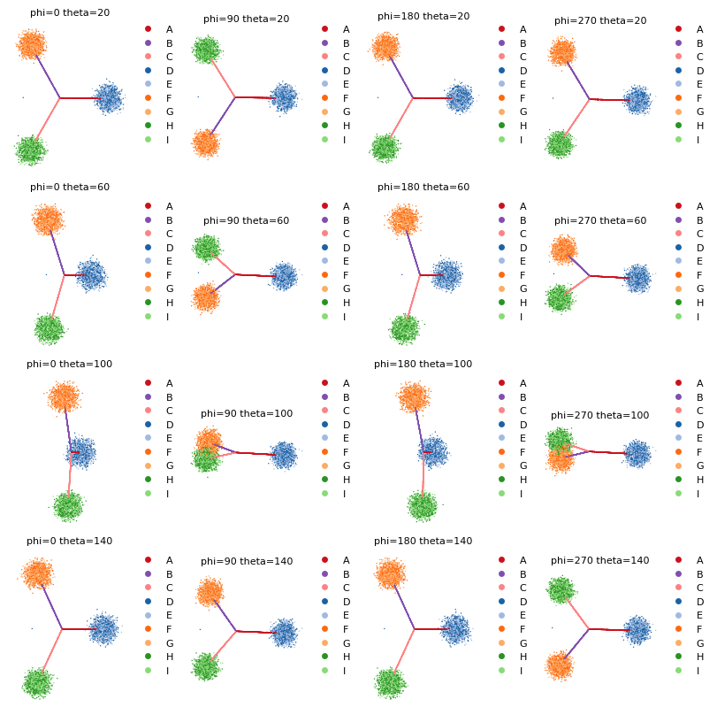
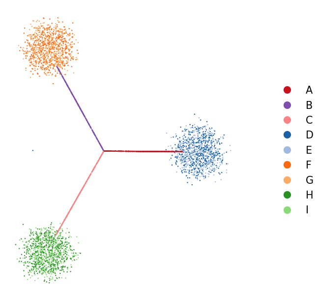
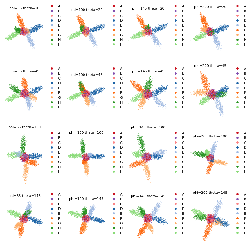
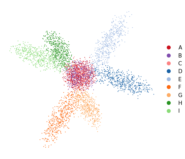
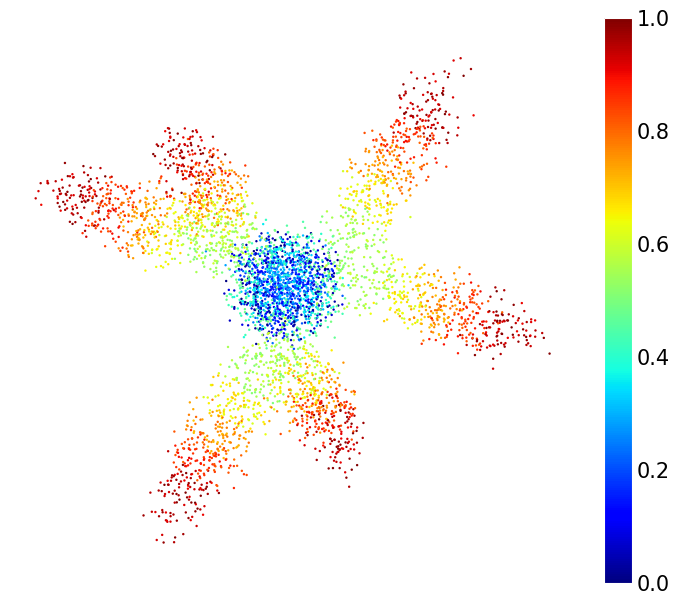
Observations are assigned to nine types A-I (simul.obs['type']) and ordered along a developmental pseudotime (simul.obs['pseudotime']). As for the previous dataset, start with visualizing single modalities.

oci.pl.projections(simul, x='modality0', c='type', phis=[0, 90, 180, 270],
                   thetas=[20, 60, 100, 140], cdict=cdict, s=1, fontsize=8,
                   figsize=(8, 8), showlegend=True, random_state=17)

oci.tl.projection(simul, x='modality0', phi=0, theta=20, random_state=17)
oci.pl.scatter(simul, x='X_proj', c='type', cdict=cdict, s=3, markerscale=2,
               fontsize=15, figsize=(7, 6), title='')

oci.pl.scatter(simul, x='X_proj', c='pseudotime', cmap='jet', s=3,
               markerscale=2, fontsize=15, figsize=(7, 6), title='')

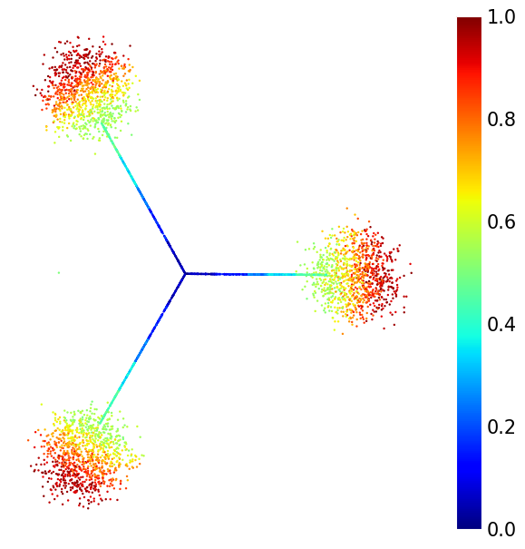
modality0 exposes types A-C as rare transitions but cannot distinguish between fates D/E, F/G, and H/I, separated in modality1.

oci.pl.projections(simul, x='modality1', c='type', phis=[55, 100, 145, 200],
                   thetas=[20, 45, 100, 145], cdict=cdict, s=1, fontsize=8,
                   figsize=(8, 8), showlegend=True, random_state=17)

oci.tl.projection(simul, x='modality1', phi=145, theta=145, random_state=17)
oci.pl.scatter(simul, x='X_proj', c='type', cdict=cdict, s=4, markerscale=2,
               fontsize=15, figsize=(7, 6), title='')

oci.pl.scatter(simul, x='X_proj', c='pseudotime', cmap='jet', s=3,
               markerscale=2, fontsize=15, figsize=(7, 6), title='')

Multimodal Diffusion Maps

Generate the MDM embedding: 1) calculate nearest neighbors, 2) compute modality weights, and 3) compute MDM components.

oci.pp.neighbors(simul, n_neighbors=60, n_jobs=50, verbose=True)
oci.tl.modality_weights(simul, random_state=17, n_jobs=50, verbose=True)
oci.tl.MDM(simul, n_components=20, unimodal_norm=False, random_state=17, n_jobs=50, verbose=True)

[modality0]     60 nearest neighbors calculated.
[modality1]     60 nearest neighbors calculated.

2025-01-29 18:32:15,654 INFO worker.py:1518 -- Started a local Ray instance.

Multimodal weights estimated.

2025-01-29 18:32:21,422 INFO worker.py:1518 -- Started a local Ray instance.

[modality0]     Unimodal Markov chain calculated.
[modality1]     Unimodal Markov chain calculated.
Multimodal Markov chain calculated.
Eigendecomposition finished.
20 Multimodal Diffusion Maps components calculated.

Visualizing MDM components

Create FLE based on the nearest neighbors graph.

oci.pp.neighbors(simul, x=['X_mdm'], n_neighbors=60, n_jobs=50, verbose=True)
oci.tl.neighbors_graph(simul, x='X_mdm', n_edges=60, verbose=True)
oci.tl.fa2(simul, n_components=2, n_iter=5000, n_jobs=50, random_state=17)

[X_mdm] 60 nearest neighbors calculated.
Nearest neighbors-based graph constructed.

Jan 29, 2025 6:32:33 PM org.netbeans.modules.masterfs.watcher.Watcher getNotifierForPlatform
INFO: Native file watcher is disabled
Jan 29, 2025 6:32:34 PM org.gephi.io.processor.plugin.DefaultProcessor process
INFO: # Nodes loaded: 4,500 (4,500 added)
Jan 29, 2025 6:32:34 PM org.gephi.io.processor.plugin.DefaultProcessor process
INFO: # Edges loaded: 270,000 (152,392 added)

*************************25%
*************************50%
*************************75%
*************************100%
Time = 28.892s

Visualize FLE.

oci.pl.scatter(simul, x='X_fa2', c='type', cdict=cdict, s=5, markerscale=2,
               fontsize=15, figsize=(8,6), title='')

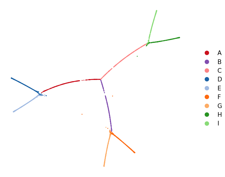
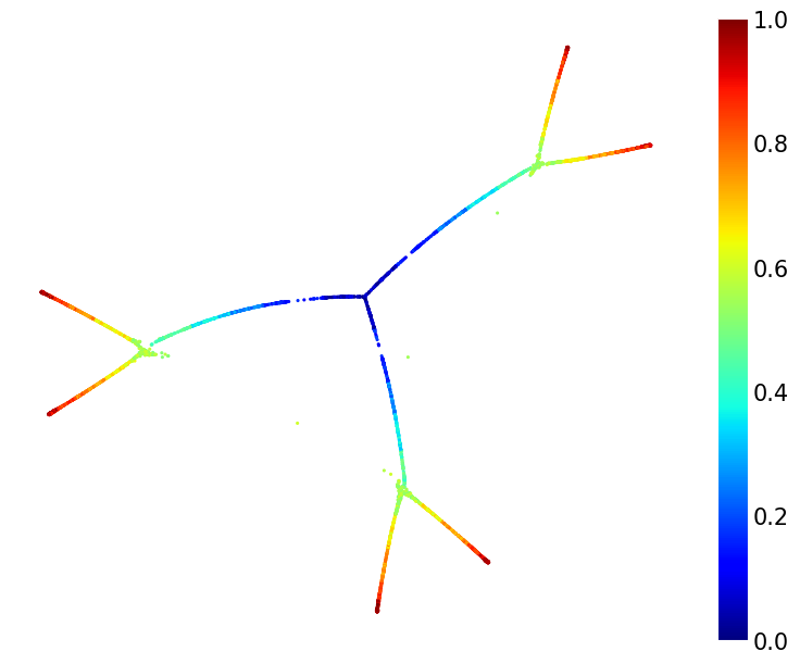
MDM managed to reconstruct developmental fates D-I and their origin A-C. Additionally, MDM preserved developmental pseudotime.

oci.pl.scatter(simul, x='X_fa2', c='pseudotime', cmap='jet', s=5,
               markerscale=2, fontsize=15, figsize=(8,6), title='')

Exploring modality weights

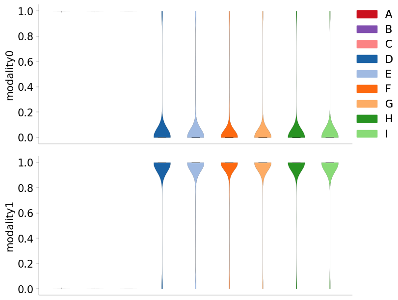
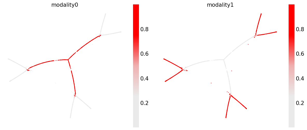
Multimodal weight distribution confirms that modality0 is more informative about types A-C and modality1 about types D-I.

oci.pl.violin(simul, groups='type', values='weights', cdict=cdict, fontsize=15,
              figsize=(8, 6))

oci.pl.scatter(simul, x='X_fa2', c='weights', cmap=cmap, s=3,
               fontsize=15, figsize=(12, 5))

It is a wrap-up of the first tutorial. You should better understand why joint multimodal visualizations unlock a new comprehension of data and how to build a basic Ocelli workflow.

In the following chapters, you will focus on single-cell data analysis.